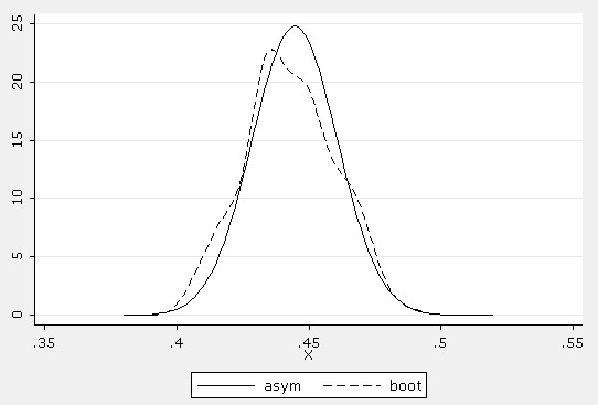
Draw the curves of the estimated
incidence indices of poverty.
|
| For this question we use
DAD and Stata 8 Steps in DAD
- From the main menu of the Spreadsheet, select the item EDIT| Edit
Last Bootstrap results
- Select the 200 estimated values and copy its in the Sheet
file2
- Select the item Edit|Set OBS : obs=200
- Use the application Distribution|Density function
- Click on button Range : Min= 0.38 | Max=0.52
- Click on button Graph
- Select the item Files|Save As and save this coordinates of
density according to the bootstrap approach.
Steps with Stata
- Load the file: File|Import|Unformatted ASCII Data (new variables
X boot)
- Generate the asymptotic distribution: gen
asym=normden(X,0.44456312, 0.01612363)
- Drawing the graph: line asym boot X, sort
|
|
|
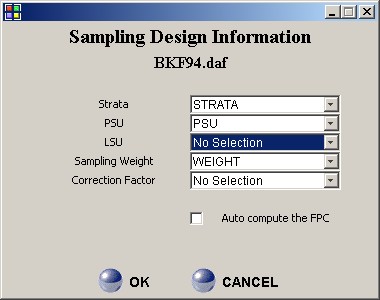
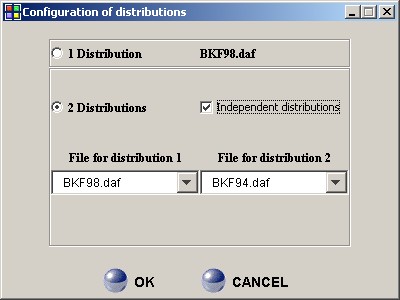
Load the file BKF98.daf in the sheet
file2
and initialise its sampling design.
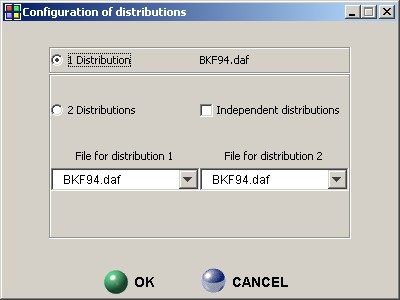
Consider that the two distributions are independent. Compute an estimate of the poverty incidence
as well as of its confidence interval when:
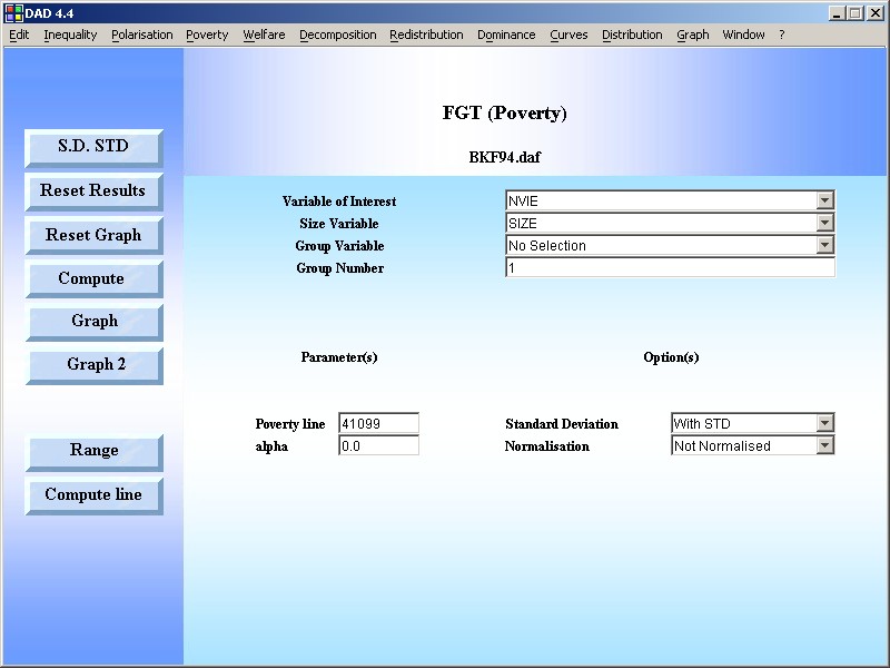
NVIE is the variable of interest
The poverty line is
72690 F CFA The asymptotic approach is
used.
|
| |
RESULTS |
FGT (Poverty)
| Session Date |
Tue Jan 04 12:28:01 EST 2005 |
| Execution Time |
0.0 sec |
| FileName |
BKF98.daf |
| OBS |
8478 |
| Sampling Weight |
WEIGHT |
| Variable of interest |
NVIE |
| Size variable |
SIZE |
| Group variable |
No Selection |
| Group Number |
1 |
| Option |
Normalised = NO |
| Parameter |
α=0 |
Index |
Estimated value |
Standard deviation |
Lower bound |
Upper bound |
Confidence Level in (%) |
FGT |
0.45267603 |
0.01092681 |
0.43125987 |
0.47409218 |
95.00000000 |
Poverty line |
72690.00000000 |
0.00000000 |
72690.00000000 |
72690.00000000 |
95.00000000 |
EDE |
0.00000000 |
0.00000000 |
0.00000000 |
0.00000000 |
95.00000000 |
|
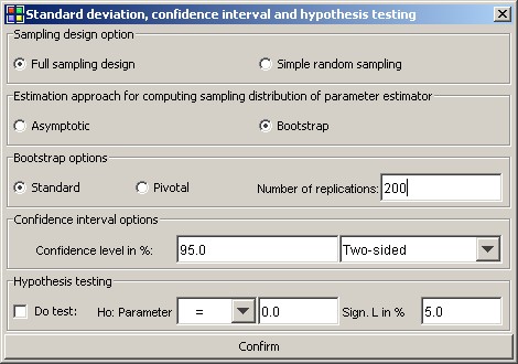
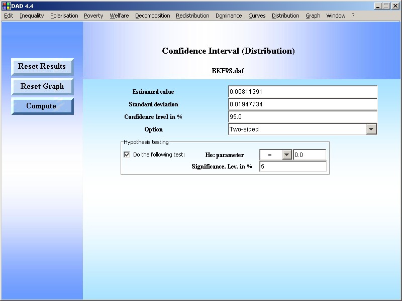
Estimate the difference and its standard
error and use the
Distribution|Confidence interval to test if the difference is null.
|
|
Use the DAD Application: Poverty|FGT Index |
|
 After choosing the appropriate variables and parameters, click on the Compute
button. |
RESULTS |
FGT (Poverty)
| Session Date |
Tue Jan 04 12:38:37 EST 2005 |
|
| Execution Time |
0.062 sec |
|
| FileName |
BKF98.daf |
BKF94.daf |
| OBS |
8478 |
8625 |
| Sampling Weight |
WEIGHT |
WEIGHT |
| Variable of interest |
NVIE |
NVIE |
| Size variable |
SIZE |
SIZE |
| Group variable |
No Selection |
No Selection |
| Index of Groups |
1 |
1 |
| Option |
Normalised = NO |
| Parameter(s) |
α=0 |
α=0 |
| Estimate |
0.45267603 |
0.44456312 |
| |
(0.01092681) |
(0.01612363) |
| Difference Index1-Index2 |
0.00811291 |
| |
(0.01947734) |
| Covariance Index1-Index2 |
0.00000000 |
| Poverty Line |
72690.00000000 |
41099.00000000 |
| |
(0.00000000) |
(0.00000000) |
|
|
Use the DAD Application: Distribution|Confidence Interval |
|
Confidence Interval (Distribution)
| Session Date |
Tue Jan 04 12:41:01 EST 2005
|
| Execution Time |
0.015 sec
|
| Sampling Weight |
WEIGHT
|
| Interval option |
Two-sided |
Estimated value
|
Standard deviation
|
Lower bound |
Upper bound |
Confidence Level in (%)
|
0.00811291 |
0.01947734 |
-0.03006197 |
0.04628779 |
95.00000000 |
Hypothesis testing: H0:parameter = 0.00000000 vs H1:
parameter ≠ 0.00000000
Result of the test
|
Significance Level in (%)
|
P-Value |
H0 is accepted
|
5.00000000 |
0.67702171
|
|